How Many Defect Images Do You Need to Train a Defect Detection Model: 25 or 12,568

Ask a machine vision vendor for a training data requirement and you get a shrug dressed as a number. A hundred images per class. Two hundred. Sometimes a thousand, which is usually a polite way of saying they do not know either.

How many defect images do you need to train a defect detection model is the question every manufacturing team eventually types into a search bar, and it deserves better than a shrug. The honest answer is a range. Published work puts the useful floor at around 25 confirmed defective samples for one tightly constrained defect on a fixed fixture. The ceiling, for a defect that looks different every time it appears, runs into five figures. Same question, two orders of magnitude apart.

What moves you along that range is not how hard the defect is to see. It is how much the defect varies. Everything else in this piece follows from that one distinction, including the reason your line probably cannot supply the images anyway.

How Many Defect Images the Published Datasets Actually Used: 25 to 12,568

The spread is not hand-waving. It sits in the datasets the field trains on.

At the low end, Tabernik, Šela, Skvarč and Skočaj built KolektorSDD from plastic embedding surfaces on electrical commutators: 399 images in total, 52 of them defective. Their segmentation and decision network reached 99.9 average precision on the full set. Then they did the experiment nobody else bothers to run. They cut the number of defective training samples per fold from 33 down to 25, 20, 15, 10 and 5, kept the test set fixed, and retrained. At 25 defective samples the method held above 99% AP with a single misclassification. At 5 defective samples it still reached roughly 96% AP. The commercial package they benchmarked against, Cognex ViDi Suite, had already dropped to 97.4% AP at 25 samples and to slightly below 90% at 5.

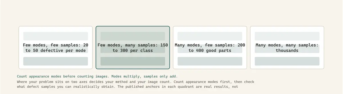
In the middle sits DAGM 2007, the weakly supervised optical inspection competition set hosted by Heidelberg's HCI. Its six development classes give you 1,000 non-defective images and 150 defective ones each. Its four competition classes give you 2,000 non-defective and 300 defective. Defects are marked only by a rough ellipse. That 150 figure is almost certainly the origin of the number your vendor quoted you.

At the top end, the Severstal steel defect challenge shipped 12,568 training images across four defect classes, 6,666 of which contain at least one defective region, and the classes are heavily unbalanced. Steel surface defects are photographed on a moving web, at scale, with variation in everything.

And running underneath all three, MVTec AD: 5,354 images across fifteen categories, of which 3,629 are training images that contain no defects at all, 467 are clean test images and 1,258 are defective test images covering 73 defect groups and 1,888 annotated defect regions. "Two orders of magnitude of defect count between KolektorSDD and Severstal, and none of them is wrong."

A crack is a geometric feature to a renderer and a specular event to a camera. Synthetic data models the first and cannot model the second.

Defect variability, not defect count, sets the number

Look at the per-category rows in the MVTec AD table and the pattern is immediate.

Look at the per-category rows in the MVTec AD table. Toothbrush: 60 training images, one defect group, 66 annotated defect regions. Cable: 224 training images, eight defect groups, 151 regions. Pill: 267 training images, seven defect groups, 245 regions. Transistor: 213 training images, four groups, only 44 regions. The table is suggestive rather than conclusive, and hazelnut is the counterexample at 391 training images for just four groups, which is a reminder that these counts record what MVTec collected and not what a method needs. The argument that follows rests on the physics, not on this table. The categories that need more data are the ones where the defect can present in more distinct ways, not the ones where the defect is subtler.

So the quantity you should be estimating is not images. It is appearance modes, and then images per mode. A mode is a distinct combination of defect physics, position, orientation and the way that combination interacts with your illumination. A scratch on a brushed aluminium housing that always runs along the grain, on a part that arrives in a fixed nest, is one mode. On KolektorSDD, which is exactly that kind of problem, 25 defective samples was enough. Treat a few dozen per mode as the starting assumption you will replace with a measured curve. Twenty to fifty examples will teach it. A scratch that can run at any angle across a curved surface, on a part that arrives at any rotation, is not one mode. It is a family, and each member of the family needs its own examples because a convolutional network does not get rotation invariance for free at the scale where a hairline defect lives.

Here is the cheap version of this measurement, and it takes an afternoon. Pull thirty confirmed rejects. Lay them on a bench under the lighting you actually intend to ship. Sort them into piles by what they look like, not by root cause. Count the piles.

Teams conflate those two taxonomies constantly, and it wrecks their data plans. Two defects with the same root cause can look nothing alike to a camera. Two with entirely different causes can be pixel-for-pixel indistinguishable. Quality engineering thinks in root causes because that is what you fix. The model only ever sees appearance. If your defect catalogue has eleven entries and your bench sort produces four piles, you are training four classes, not eleven, and your image budget just dropped by more than half.

On a line running at high yield the defects do not exist yet

This is where the arithmetic turns hostile, and it is the part vendors skip.

Siemens published 132 days of automated optical inspection data from a single surface-mount line in Germany. The file holds 440,274 soldering spots. Every one of them is a point the AOI machine flagged as defective and escalated to a human at the manual inspection station. Boards the machine passed are not in the file at all.

Of those 440,274 escalations, 4,622 were confirmed true defects. The other 435,652 were false calls. That is 1.05% real, 98.95% good product wrongly condemned by the inspection system.

Sit with the first number for a second. Four thousand six hundred confirmed defects, across every defect type on the line, over a recording phase of 132 days. About 35 a day, total. Split that across your defect classes and the rarest class might produce a handful a week. If your data plan says 200 images of that class, you are proposing to wait roughly a year, during which the solder paste supplier changes, a feeder gets replaced and a lamp ages out. The process you were sampling no longer exists by the time you have sampled it.

Buda, Maki and Mazurowski ran the systematic study of what that imbalance does to convolutional networks, in Neural Networks in 2018. Their findings are useful and limited in the same breath: the effect of imbalance on performance is detrimental, oversampling emerged as dominant in almost all scenarios and, unlike classical models, oversampling does not cause CNNs to overfit, and thresholding should be applied to compensate for prior class probabilities. Real guidance. But oversampling twelve images of a defect does not manufacture a thirteenth appearance mode. It only stops the loss function from ignoring the twelve you have.

The second number in the Siemens file is the one that connects this to everything I have written about false rejects. "Nearly 436,000 records of good product that a deployed inspection system called bad. Siemens released the AOI measurements rather than the underlying images, but on your own line that same pool is two things at once: the actual business problem, and a free corpus of labelled normal data." Which points at the method you should try first.

One-class methods let you start with the parts you already have

MVTec AD, the benchmark that defines this field, never shows a model a defect during training. Every one of its 3,629 training images is defect-free. Per category, methods get between 60 normal images (toothbrush) and 391 (hazelnut).

PatchCore, from Roth and colleagues at CVPR 2022, reports 99.0% image-level AUROC on MVTec AD using the full normal training set, and up to 99.6% in the paper's strongest configuration. The interesting table is the low-shot one. With 1 normal image: 83.4% AUROC. With 5: 90.8%. With 10: 93.6%. With 16: 95.4%. With 50: 97.5%.

Sixteen photographs of a good part gets you to 95.4% on a curated benchmark. That is not a production system, but it is a Tuesday afternoon, and it answers a question no amount of arguing about image budgets will answer: is this defect separable at all under my current optics.

Two costs come with going one-class, and you should price them before you commit.

The first is that an anomaly score is not a disposition. You get a number, not a class, so you have to pick a threshold, and the threshold is exactly where your false-reject rate lives. AUROC conceals this completely because it integrates across every threshold, including thresholds that would reject a third of your production. When someone quotes you an AUROC, the number you actually needed was recall at a fixed false-reject budget. Ask for that one instead, and watch what happens to the confidence in the room.

The second is that a one-class model flags anything unusual, and legitimate variation you failed to show it counts as unusual. A new material lot. A different operator's part placement. A lamp at 80% of its rated output. All of it reads as anomalous, which means your normal set has to be sampled across shifts, lots and lamp ages, not collected in one clean hour on a Wednesday.

Synthetic defects work until the physics of the defect changes

The obvious response to defect scarcity is to manufacture the images. Sometimes this works far better than it has any right to.

DRAEM, from Zavrtanik, Kristan and Skočaj at ICCV 2021, trains on anomaly-free images plus synthetic anomalies generated by thresholding Perlin noise and blending in a patch of unrelated texture. The synthetic anomalies look nothing like real defects. The method still reaches 98.0 image-level AUROC and 97.3 pixel-level AUROC on MVTec AD. What the network learns is not what a defect looks like but where the decision boundary between reconstructable and non-reconstructable content sits.

Now the failure. A 2025 study on photolithographic patterns trained detection models entirely on synthetic scanning electron microscope images with autonomously generated annotations. On synthetic test data, YOLOv8 reached 96% mean average precision. On real SEM images, the same model detected bridge defects at 84.6% and break defects at 78.3%.

"That paper does not isolate a cause, so here is the mechanism I would test on your own parts. Synthetic generators model the defect's geometry. They do not model how that geometry registers on your particular sensor. In visible light a crack is a geometric feature to a renderer and a specular event to a camera, and whether it registers at all depends on the angle between the surface normal, the light source and the sensor, and on whether you are working in dark field, bright field or backlight." Whether it registers at all depends on the angle between the surface normal, the light source and the sensor, and on whether you are working in dark field, bright field or backlight. This is the same argument I have made about lighting, arriving from the opposite direction. If the optics do not make the defect visible, no volume of synthetic data will invent it. If the optics do make it visible, you need fewer real images than you feared.

So the practical boundary: use synthetic generation to vary position, scale, rotation and background for modes you have already photographed at least once. Do not use it to conjure a mode you have never seen. The first is augmentation. The second is a hypothesis wearing a dataset's clothes.

The strongest case for a fixed number, and exactly where it holds

The honest counter-argument to everything above is that sometimes 150 per class is simply correct, and the vendor is not shrugging at all. They are quoting DAGM, and DAGM was a real competition that real methods solved.

"Look at the conditions those classes satisfy. The DAGM images are artificially generated, one texture model and one defect model per class, so the appearance of a defect is reproducible by construction rather than by fixturing. One defect family per class. No part rotation, because there is no part and no camera, only synthesised material. Under those conditions a few hundred defective images per class was enough to run an international competition on. If your problem genuinely has that much repeatability you can borrow the number, but note what is doing the work: DAGM is repeatable because nothing in it varies, which is the one property no real line has." Under those conditions 150 defective images per development class was enough to build a benchmark on, and 300 per competition class was enough to run an international contest on.

The qualifying condition is not simplicity. It is repeatability. The requirement is that the image of the defect be reproducible, which is a statement about your fixturing and your lighting, not about your defect.

And there is a counter to the counter, published last year. MVTec AD 2 assembled eight scenarios with more than 8,000 high-resolution images, deliberately including transparent and overlapping objects, dark-field and backlight illumination, high variance within the normal data and extremely small defects. Critically, the test images were captured under lighting conditions not necessarily present in the training data. Current state-of-the-art methods stay below 60% average AU-PRO on it.

Read that as a warning about borrowed numbers. "Read that as a warning about borrowed numbers. On the original MVTec AD the best published AU-PRO is 97.8%. On MVTec AD 2 the best is 58.7%. The paper spreads the blame across transparency, backlight and dark-field imaging, high variance in the normal data and very small defects, and it isolates the lighting shift as costing the average method around 11 points on its own. Every sample-size figure you have ever been quoted was measured under conditions that were held constant, and yours will not be." Every sample-size figure you have ever been quoted was measured under conditions that were held constant, and yours will not be.

Stage the pilot so it produces your number instead of someone else's

Here is the sequence I would run, and it gets you a defensible number in about two weeks using data you already own.

Freeze the optics before you collect a single training image. Lighting geometry, exposure, working distance, part presentation, all locked and documented. Every image collected before the optics are frozen becomes worthless the moment they change, and they always change. This is the highest-value week of the whole project and not one hour of it is machine learning.

Sort before you count. The bench exercise from earlier gives you your mode count. That number, not a vendor's, sets the shape of everything downstream.

Harvest normals for free. Every part the line passes is a labelled normal image that costs you nothing but storage. Take a few hundred per variant, spread deliberately across shifts, operators, material lots and lamp ages, so the normal set contains the legitimate variation the model must learn to ignore.

Build the one-class baseline before buying anything. Two hundred normal images and a memory-bank method will tell you within a day whether your defects separate under your current optics. If they do not, the correct next purchase is a different light, not more defect images, and you have just saved a quarter of pointless data collection.

Then fit a learning curve rather than guessing a target. Hold out a fixed test set. Train at 5, 10, 20, 40 and all available defective samples, three random seeds at each point to get error bars, and plot recall at a fixed false-reject rate rather than AUROC. Fit an inverse power law to those points and extrapolate. Figueroa and colleagues set out this exact procedure for classification sample size in BMC Medical Informatics and Decision Making in 2012, fitting an inverse power law to a learning curve built from a small annotated set and using it to predict performance at larger sample sizes. The statistics transfer directly to defect detection. I have not run this on your parts and I will not pretend a number for them. The point of the procedure is that it produces one, for your defect, with data you have already collected.

Make the held-out set adversarial about conditions, not only about defects. A lamp near end of life. A different shift. A material lot change. MVTec AD 2 is the published evidence that a test set holding lighting constant will flatter you, and a flattering test set is how a pilot passes and a deployment fails.

Finally, read the slope rather than the height. If recall is still climbing steeply at your current sample count, more images is the right investment and the curve tells you roughly how many. If it has flattened at 92% and you need 99%, no quantity of additional images will close that gap. The residual error is either a mode you have never captured or an imaging problem, and both need a different intervention entirely.

The number to ask a vendor for is not a number of images

When someone quotes you a training set size, three follow-up questions do all the work. At what false-reject rate was that recall measured. Across how many visually distinct defect appearances. Under how many lighting conditions, and were any of them absent from the training data.

A vendor who answers "200 per class" before asking what your defect looks like has told you something valuable, just not what they intended. They have told you they have not seen your part.

The sample size is not a property of defect detection as a discipline. It is a property of your defect's variability, your optics and your yield, and those three things only exist in one place. Every team I have pushed through the staged pilot instead of handing a number was irritated for about a fortnight. Then they had a number, and it was theirs, and nobody could sell them a different one.

Tools referenced

Roboflow, reviewed here: Roboflow review.

Label Studio, reviewed here: Label Studio review.

Sources

Tabernik, Šela, Skvarč & Skočaj, Segmentation-Based Deep-Learning Approach for Surface-Defect Detection (KolektorSDD sample-size experiments): https://arxiv.org/abs/1903.08536: https://arxiv.org/abs/1903.08536

Bergmann et al., MVTec AD: A Comprehensive Real-World Dataset for Unsupervised Anomaly Detection (per-category statistics table): https://www.mvtec.com/fileadmin/Redaktion/mvtec.com/05_research_teaching/datasets/mvtec_ad.pdf

Heckler et al., The MVTec AD 2 Dataset: Advanced Scenarios for Unsupervised Anomaly Detection (lighting-shift test scenarios): https://arxiv.org/abs/2503.21622

Roth et al., Towards Total Recall in Industrial Anomaly Detection (PatchCore, including low-shot results): https://arxiv.org/abs/2106.08265

Data of automated optical inspection of surface-mounted technology electronic production, Siemens AG, 132-day AOI dataset: https://pmc.ncbi.nlm.nih.gov/articles/PMC10847760/

Zavrtanik, Kristan & Skočaj, DRAEM: A Discriminatively Trained Reconstruction Embedding for Surface Anomaly Detection: https://arxiv.org/abs/2108.07610

Defect Detection in Photolithographic Patterns Using Deep Learning Models Trained on Synthetic Data (synthetic-to-real gap): https://arxiv.org/abs/2505.10192

DAGM 2007, Weakly Supervised Learning for Industrial Optical Inspection, Heidelberg Collaboratory for Image Processing: https://hci.iwr.uni-heidelberg.de/content/weakly-supervised-learning-industrial-optical-inspection