Self-Balancing Robot Simulation: What Transfers and What Does Not

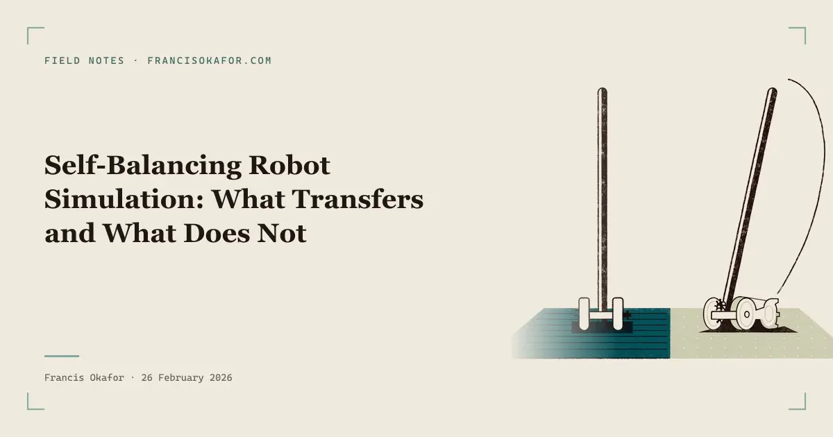
Self-balancing robot simulation is the first thing most engineers reach for, and it is the right instinct for the wrong reason. The instinct is sound: the maths is cheap and the hardware is not. The wrong reason is the belief that a controller which balances in the simulator is a controller that balances.

It is not. What simulation gives you is structural. Does the loop close. Is the state you can actually measure enough to close it. Roughly how fast does the loop have to run relative to the physics. What it does not give you is a number you can flash to the board.

The failure mode I keep meeting is a team that spent three weeks on the model and ten minutes on the sensor, then spent another three weeks wondering why the gains were wrong. The reality gap is not one big modelling mistake. It is six small ones, each of which the simulator quietly sets to zero, compounding once per control cycle at a few hundred cycles per second.

The inverted pendulum as the standard model

The inverted pendulum earned its place in every control curriculum by being the smallest system that is unstable, underactuated and nonlinear at the same time. Linearise about the upright equilibrium and you get a pole in the right half plane. The practical meaning of that pole is that there is no do-nothing fallback. Open the loop and the error grows exponentially. A quadrotor hovers badly when the controller is off; a pendulum simply falls.

The cart-pole formulation has been a shared benchmark since Barto, Sutton and Anderson used it in 1983 as the test problem for a learning controller that had no model of the plant and only a failure signal to learn from. It stuck because it is small enough to reason about and hard enough to be interesting.

A two-wheeled balancer is the same skeleton with wheel inertia and motor dynamics bolted on. It also inherits a property that surprises people the first time: to drive forward, the wheels must first drive backward, so the body tips into the direction of travel. That is non-minimum phase behaviour in the base-position channel. A position loop that refuses to tolerate a wrong-way transient will fight the physics and lose.

Everything about timing is measured against the pendulum time constant, which scales as the square root of length over gravity. For a chassis with its centre of mass 100 mm above the wheel axle, that is roughly 0.10 seconds. Your loop rate, filter bandwidth and total latency budget all live inside that number, not inside a round figure someone posted on a forum.

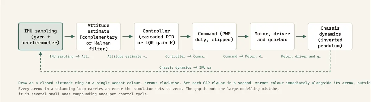
The simulator is not lying to you. It is telling you the truth about a robot you did not build.

PID tuned in simulation versus LQR, and what each assumes

PID assumes a single input, a single output and no model. That is its selling point and its trap. A balancer needs at least two loops: an inner angle loop, and an outer wheel-velocity or position loop whose output is a tilt setpoint. Cascade control assumes time-scale separation between the two. In simulation you can violate that separation freely, because there is no noise to punish you and no phase lag from a filter you have not written yet.

LQR assumes more and admits it. A linear model about the operating point, a quadratic cost, full state feedback and no input limits. Solve the algebraic Riccati equation, get a gain matrix, done. Two of those assumptions break on any real balancer. You do not have full state, you have a noisy rate gyro and an accelerometer, so you need an estimator, and the estimator's dynamics are now inside the loop you just proved stable. And input limits are real, whereas LQR optimality is derived over unbounded control effort. The instant your PWM clips, the guarantee is void and the integral action can wind up against a wall.

Here is the tradeoff nobody puts in the README. LQR does not remove work, it relocates it. PID lets you tune what you cannot model. LQR lets you model what you cannot tune. On a small build the term you are least likely to know accurately is the body inertia about the axle, and LQR is precisely the method that cares most about that term. Simulation flatters both methods equally, because in simulation the inertia you assumed and the inertia the plant has are literally the same variable.

Where the simulator is optimistic

Friction first. General-purpose engines approximate the Coulomb friction cone and relax the strict complementarity condition to keep the solve convex and fast. MuJoCo documents this openly, describes its soft contact model as deliberately dropping strict complementarity, and lists velocity-dependent slip effects during friction transitions among the phenomena it ignores. For a balancer, the term that matters is not tyre grip anyway. It is stiction in the gearbox and deadband in the motor driver. Below some command value the wheels do not turn at all, so the controller sits in a small limit cycle around upright, buzzing. In simulation the motor produced torque proportional to command all the way down to zero, so the buzz never appeared.

Sensor noise second, and the interesting part is not the noise. Take a commodity IMU: the MPU-6050 product specification gives a gyroscope rate noise spectral density of 0.005 degrees per second per root hertz and a total RMS noise of 0.05 degrees per second. That is small. Bias is the problem, because the integrated gyro angle drifts and the accelerometer is what pulls it back. But an accelerometer measures specific force, not gravity. It reads chassis acceleration too, and chassis acceleration is nonzero exactly when the robot is correcting. Your tilt reference is corrupted by the control action that produced it. This coupling is the single most common thing missing from a hobby simulation, and it is the one that changes the character of the closed loop rather than just its margins.

Then actuator saturation. Brushed DC torque falls with speed, so the torque available during a fast recovery is not the torque on the stall curve. Battery voltage sags under load and again across the discharge curve, so the gains you tuned on a full pack are not the gains you have on a flat one. Add gearbox backlash, encoder quantisation and the phase lag of whatever complementary or Kalman filter you put on the front. Every millisecond of group delay eats phase margin you thought you had.

Last, jitter. The simulator advances by exactly dt, forever. A general-purpose Linux scheduler does not, which is why real-time preemption and bare-metal microcontrollers exist. A loop that runs at a nominal period with occasional long steps is not the loop you designed, and the discrepancy shows up as an effective delay that varies. The version of this I would not ship again is a balancing loop sharing a core with a logging thread and a network stack, on a stock kernel, tuned against a simulation with zero jitter.

Domain randomisation and where it stops paying

The standard answer to all of the above is domain randomisation. Sample the physical parameters per episode, train across the distribution rather than at a point and hope the real system falls inside. OpenAI's in-hand manipulation work is the canonical demonstration, randomising friction coefficients and object properties in physics and randomising textures, lighting and camera pose for the vision network, then transferring to a physical hand with no real-world training.

It works, within two limits that matter for a small build. The first is that you can only randomise parameters your model contains. Widening the range on a friction coefficient does nothing about a friction model with no stiction term, and no range is wide enough to reach a phenomenon that is absent. The alternative that actually works is measurement. When Hwangbo and colleagues transferred locomotion policies to ANYmal in Science Robotics in 2019, they did not randomise their way past the series-elastic actuators, they trained a network on hardware data to predict actuator response and put that model inside the simulator.

The second limit is what randomisation costs. Chen and colleagues analysed domain randomisation formally, modelling the simulator as an MDP with tunable parameters, and derived bounds on the sim-to-real gap that hold without real-world samples under mild conditions. Their analysis makes the mechanism explicit: the true parameters are hidden, so the problem is effectively partially observed and history-dependent policies matter. A memoryless controller facing a wide randomisation range has exactly one strategy available, which is to be conservative everywhere. On a balancer that produces a policy which survives and does not perform. Sluggish. Wide deadzone around upright. Fine on carpet, terrible on a ramp.

What self-balancing robot simulation genuinely answers

The honest split runs along the line between structural and quantitative. Simulation answers structural questions well. Is the system controllable with the actuators you have and observable with the sensors you chose. Does a cascade structure work at all, or does the outer loop need to be something other than a PI on wheel speed. What order of magnitude of loop rate does the time constant demand. What does the swing-up energy trajectory look like, and will it slam the chassis into the desk. It also gives you a regression harness, so a refactor cannot silently invert a sign, and sign errors in gyro integration account for more failed first flights than any subtlety in the gain matrix.

Simulation does not answer quantitative questions about your hardware. Not the gain values. Not the torque headroom. Not the latency budget, the deadband, the real noise floor or how the whole thing behaves at half battery. If a number in your controller came out of a simulator and was never checked against the rig, treat it as a starting guess with a plausible order of magnitude and nothing more.

The case for skipping simulation on a small rig

The strongest counter-argument is one I mostly agree with, and it is worth stating at full strength rather than as a strawman. A desktop balancer falling 200 mm onto foam is an almost free failure. Failures that cost nothing are the fastest teachers available, and a physical rig delivers them at a rate no simulator matches, with perfect fidelity, including the failures you did not think to model. A week spent building a scene in a physics engine is a week not spent discovering that your motor driver has a deadband nobody documented.

Model building also has a seductive failure mode. You tune the model until it agrees with the video, which is curve fitting dressed as physics, and it produces a simulator that reproduces the one experiment you already ran. For a first balancer I would put the time into instrumentation instead: log the raw gyro, the commanded PWM, the encoder counts and the loop period, all timestamped, and plot them. That is system identification, and it is what makes a simulator worth building afterwards rather than beforehand.

What flips the calculus is cost of failure and sample count. Hardware heavy enough to hurt when it falls. Stored energy that is dangerous. A learning-based controller that needs millions of episodes and cannot get them on a rig. More than one person working on the controller at once. Anything that has to run unattended in CI. For a two-wheeled robot on a desk, none of those apply, and the argument for hardware first is strong.

Simulator options, and the case for no simulator at all

For a linearised balancer with four or six states, a plain ODE integrator in Python or a Simulink model is often the correct tool and a physics engine is overkill. You wrote the equations yourself, so you know exactly which terms are missing, which is more than you can say for a scene file.

When you do want contact and a full rigid body, the practical options divide by what they optimise for. MuJoCo is the default for contact-rich work and control research, with MJX for GPU-parallel rollouts underneath MuJoCo Playground, which won the outstanding demo paper award at RSS 2025 and packages training environments for quadrupeds, humanoids, dexterous hands and arms with the stated goal of zero-shot sim-to-real transfer, trainable in minutes on a single GPU. Isaac Sim with Isaac Lab is where you go for photorealistic perception and thousands of parallel environments, at the cost of a heavy stack. Gazebo is the answer if you are already committed to ROS 2, and the release schedule matters more than people expect: Harmonic and Jetty are long-term support, Jetty is supported to May 2031, and Ionic reaches end of life in December 2026, so start on an LTS. PyBullet and Webots are lighter and friendlier for a first project. Drake is the one to reach for when your problem is control and identification rather than pixels.

LLM assistants are genuinely useful for the tedious part of this. Claude, or GitHub Copilot inside Cursor, will produce MJCF scaffolding or a Lagrangian derivation faster than you will by hand, and the derivation is checkable, which is the property that makes it safe to accept. What you will also get is a friction and actuator model that is confidently wrong in a specific way: it will be the textbook model rather than yours, with the deadband, backlash and torque-speed curve all absent. Check every parameter against the datasheet and the rig, never against the generated comment that explains it.

The gap migrates, it does not close

The simulator is not lying to you. It is telling you the truth about a robot you did not build. Each year the engines get better at the things they already represent: contact solvers, learned actuator models, GPU-parallel rollouts, randomisation schedules that adapt themselves.

Which leaves an uncomfortable observation. The residual gap on a small machine is increasingly not physics at all. It is the scheduler that missed a deadline, the connector that worked loose, the pack halfway down its discharge curve and the motor that came off the reel a little weaker than its twin. No simulator will grow a feature for those, because they are not modelling problems. If that is where the remaining error lives, then effort spent making the physics more faithful is effort spent improving the part of the model that was already close to right.

Tools referenced

Claude, reviewed here: Claude review.

GitHub Copilot, reviewed here: GitHub Copilot review.

Cursor, reviewed here: Cursor review.

Sources

Barto, Sutton & Anderson (1983), Neuronlike adaptive elements that can solve difficult learning control problems, IEEE Trans. SMC: https://ui.adsabs.harvard.edu/abs/1983ITSMC..13..834B/abstract

MuJoCo documentation: computation, contact model and friction cones: https://mujoco.readthedocs.io/en/stable/computation/index.html

MuJoCo Playground (RSS 2025 Outstanding Demo Paper): https://playground.mujoco.org/

Gazebo release schedule and support dates: https://gazebosim.org/docs/latest/releases/

MPU-6000/MPU-6050 Product Specification, rev 3.4 (gyroscope noise figures): https://www.cdiweb.com/datasheets/invensense/mpu-6050_datasheet_v3%204.pdf

OpenAI et al. (2018), Learning Dexterous In-Hand Manipulation (domain randomisation): https://arxiv.org/abs/1808.00177

Hwangbo et al. (2019), Learning agile and dynamic motor skills for legged robots, Science Robotics: https://www.science.org/doi/10.1126/scirobotics.aau5872

Chen et al. (2021), Understanding Domain Randomization for Sim-to-real Transfer: https://arxiv.org/abs/2110.03239